9.0 KiB
9.0 KiB
Power for mixed-effects models
Last modified: 2026-01-09
library(lattice)
library(lme4)
Reanalysis
Application context: Depression and type of diagnosis
- Reisby et al. (1977) studied the effect of Imipramin on 66 inpatients treated for depression
- Depression was measured with the Hamilton depression rating scale
- Patients were classified into endogenous and non-endogenous depressed
- Depression was measured weekly for 6 time points
Data: reisby.txt
dat      <- read.table("../data/reisby.txt", header = TRUE)
dat$id   <- factor(dat$id)
dat$diag <- factor(dat$diag, levels = c("nonen", "endog"))
dat      <- na.omit(dat)     # drop missing values
head(dat, n = 13)
##     id hamd week  diag endweek
## 1  101   26    0 nonen       0
## 2  101   22    1 nonen       0
## 3  101   18    2 nonen       0
## 4  101    7    3 nonen       0
## 5  101    4    4 nonen       0
## 6  101    3    5 nonen       0
## 7  103   33    0 nonen       0
## 8  103   24    1 nonen       0
## 9  103   15    2 nonen       0
## 10 103   24    3 nonen       0
## 11 103   15    4 nonen       0
## 12 103   13    5 nonen       0
## 13 104   29    0 endog       0
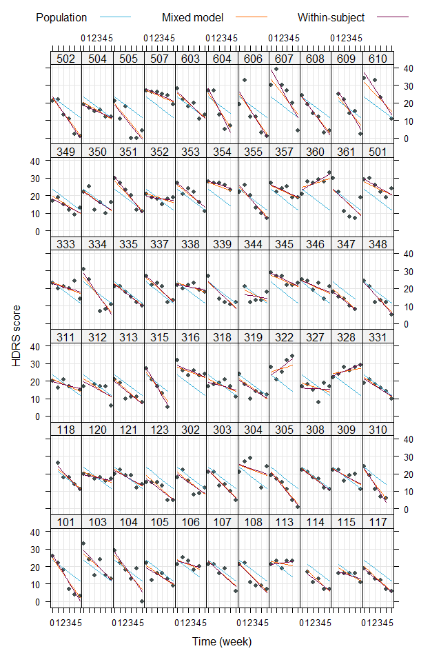
xyplot(hamd ~ week | id, data = dat, type=c("g", "r", "p"),
  pch = 16, layout = c(11, 6), ylab = "HDRS score", xlab = "Time (week)")

Random-intercept model
\begin{aligned}
Y_{ij} &= \beta_0 + \beta_1 \, \mathtt{week}_{ij}
        + \upsilon_{0i}
        + \varepsilon_{ij} \\
\upsilon_{0i} &\sim N(0, \sigma^2_{\upsilon_0}) \text{ i.i.d.} \\
\mathbf{\varepsilon}_i &\sim N(0, \, \sigma^2)  \text{ i.i.d.} \\
i &= 1, \ldots, I, \quad j = 1, \ldots n_i
\end{aligned}
m1 <- lmer(hamd ~ week + (1 | id), data = dat, REML = FALSE)
summary(m1)
## Linear mixed model fit by maximum likelihood  ['lmerMod']
## Formula: hamd ~ week + (1 | id)
##    Data: dat
##
##       AIC       BIC    logLik -2*log(L)  df.resid
##    2293.2    2308.9   -1142.6    2285.2       371
##
## Scaled residuals:
##     Min      1Q  Median      3Q     Max
## -3.1739 -0.5876 -0.0342  0.5465  3.5297
##
## Random effects:
##  Groups   Name        Variance Std.Dev.
##  id       (Intercept) 16.16    4.019
##  Residual             19.04    4.363
## Number of obs: 375, groups:  id, 66
##
## Fixed effects:
##             Estimate Std. Error t value
## (Intercept)  23.5518     0.6385   36.88
## week         -2.3757     0.1350  -17.60
##
## Correlation of Fixed Effects:
##      (Intr)
## week -0.524
Random-slope model
\begin{aligned}
Y_{ij} &= \beta_0 + \beta_1 \, \mathtt{week}_{ij}
        + \upsilon_{0i} + \upsilon_{1i}\, \mathtt{week}_{ij}
        + \varepsilon_{ij} \\
\begin{pmatrix} \upsilon_{0i}\\ \upsilon_{1i} \end{pmatrix} &\sim
   N \left(\begin{pmatrix} 0\\ 0 \end{pmatrix}, \,
           \mathbf{\Sigma}_\upsilon =
\begin{pmatrix}
          \sigma^2_{\upsilon_0} & \sigma_{\upsilon_0 \upsilon_1} \\
          \sigma_{\upsilon_0 \upsilon_1} & \sigma^2_{\upsilon_1} \\
\end{pmatrix} \right)
      \text{ i.i.d.} \\
\mathbf{\varepsilon}_i &\sim N(\mathbf{0}, \, \sigma^2 \mathbf{I}_{n_i})
      \text{ i.i.d.} \\
i &= 1, \ldots, I, \quad j = 1, \ldots n_i
\end{aligned}
m2 <- lmer(hamd ~ week + (week | id), data = dat, REML = FALSE)
summary(m2)
## Linear mixed model fit by maximum likelihood  ['lmerMod']
## Formula: hamd ~ week + (week | id)
##    Data: dat
##
##       AIC       BIC    logLik -2*log(L)  df.resid
##    2231.0    2254.6   -1109.5    2219.0       369
##
## Scaled residuals:
##     Min      1Q  Median      3Q     Max
## -2.7460 -0.5016  0.0332  0.5177  3.6834
##
## Random effects:
##  Groups   Name        Variance Std.Dev. Corr
##  id       (Intercept) 12.631   3.554
##           week         2.079   1.442    -0.28
##  Residual             12.216   3.495
## Number of obs: 375, groups:  id, 66
##
## Fixed effects:
##             Estimate Std. Error t value
## (Intercept)  23.5769     0.5456   43.22
## week         -2.3771     0.2087  -11.39
##
## Correlation of Fixed Effects:
##      (Intr)
## week -0.449
Partial pooling
indiv <- unlist(
  sapply(unique(dat$id),
         function(i) predict(lm(hamd ~ week, dat[dat$id == i, ])))
)

xyplot(hamd + predict(m2, re.form = ~ 0) + predict(m2) + indiv ~ week | id,
  data = dat, type = c("p", "l", "l", "l"), pch = 16, grid = TRUE,
  distribute.type = TRUE, layout = c(11, 6), ylab = "HDRS score",
  xlab = "Time (week)",
  # customize colors
  col = c("#434F4F", "#3CB4DC", "#FF6900", "#78004B"),
  # add legend
  key = list(space = "top", columns = 3,
             text = list(c("Population", "Mixed model", "Within-subject")),
             lines = list(col = c("#3CB4DC", "#FF6900", "#78004B")))
  )
By-group random-slope model
m3 <- lmer(hamd ~ week + diag + (week | id), data = dat, REML = FALSE)
m4 <- lmer(hamd ~ week * diag + (week | id), data = dat, REML = FALSE)
anova(m3, m4)
## Data: dat
## Models:
## m3: hamd ~ week + diag + (week | id)
## m4: hamd ~ week * diag + (week | id)
##    npar    AIC    BIC  logLik -2*log(L)  Chisq Df Pr(>Chisq)
## m3    7 2228.9 2256.4 -1107.5    2214.9
## m4    8 2230.9 2262.3 -1107.5    2214.9 0.0042  1     0.9486
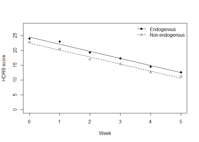
Means and predicted HDRS score by group
dat2 <- aggregate(hamd ~ week + diag, dat, mean)
dat2$m4 <- predict(m4, newdata = dat2, re.form = ~ 0)

plot(m4 ~ week, dat2[dat2$diag == "endog", ], type = "l",
     ylim=c(0, 28), xlab="Week", ylab = "HDRS score")
lines(m4 ~ week, dat2[dat2$diag == "nonen", ], lty = 2)
points(hamd ~ week, dat2[dat2$diag == "endog", ], pch = 16)
points(hamd ~ week, dat2[dat2$diag == "nonen", ], pch = 21, bg = "white")
legend("topright", c("Endogenous", "Non endogenous"),
       lty = 1:2, pch = c(16, 21), pt.bg = "white", bty = "n")
Gory details
fixef(m4)
##    (Intercept)           week      diagendog week:diagendog
##    22.47626332    -2.36568746     1.98802087    -0.02705576
getME(m4, "theta")
##      id.(Intercept) id.week.(Intercept)             id.week
##           0.9760823          -0.1175194           0.3951992
t(chol(VarCorr(m4)$id))[lower.tri(diag(2), diag = TRUE)] / sigma(m4)
## [1] 0.9760823 -0.1175194 0.3951992
Power simulation
Setup
## Study design and sample sizes
n_week <- 6
n_subj <- 80
n <- n_week * n_subj

dat <- data.frame(
     id = factor(rep(seq_len(n_subj), each = n_week)),
   week = rep(0:(n_week - 1), times = n_subj),
  treat = factor(rep(0:1, each = n/2), labels = c("ctr", "trt"))
)

## Fixed effects and variance components
beta <- c(22, -2, 0, -1)
Su <- matrix(c(12, -1.5, -1.5, 2), nrow = 2)
se <- 3.5
Power
pval <- replicate(200, {

  # Data generation
  means <- model.matrix( ~ week * treat, dat) %*% beta
  ranu <- MASS::mvrnorm(n_subj, mu = c(0, 0), Sigma = Su)
  e <- rnorm(n_subj * n_week, mean = 0, sd = se)

  y <- means + ranu[dat$id, 1] + ranu[dat$id, 2] * dat$week + e

  # Fitting model to test H0
  m0 <- lmer(y ~ week + treat + (1 + week | id), data = dat, REML = FALSE)
  m1 <- lmer(y ~ week * treat + (1 + week | id), data = dat, REML = FALSE)
  anova(m0, m1)["m1", "Pr(>Chisq)"]
  }
)

mean(pval < 0.05)
## [1] 0.805
Parameter recovery
par <- replicate(200, {

  means <- model.matrix( ~ week * treat, dat) %*% beta
  ranu <- MASS::mvrnorm(n_subj, mu = c(0, 0), Sigma = Su)
  e <- rnorm(n_subj * n_week, mean = 0, sd = se)

  y <- means + ranu[dat$id, 1] + ranu[dat$id, 2] * dat$week + e

  m1 <- lmer(y ~ week * treat + (1 + week | id), data = dat, REML = FALSE)
  list(fixef = fixef(m1), theta = getME(m1, "theta"), sigma = sigma(m1))
  }, simplify = FALSE
)

rowMeans(sapply(par, function(x) x$fixef))
##   (Intercept)          week      treattrt week:treattrt
##   22.00069056   -1.98276116    0.03001846   -1.03298775
rowMeans(sapply(par, function(x) x$theta))
##      id.(Intercept) id.week.(Intercept)             id.week
##           0.9767601          -0.1180799           0.3763657
mean(sapply(par, function(x) x$sigma))
## [1] 3.479607
beta
## [1] 22 -2 0 -1
Lt <- chol(Su)
t(Lt)[lower.tri(Lt, diag = TRUE)] / se
## [1] 0.9897433 -0.1237179 0.3846546
se
## [1] 3.5
References
Reisby, N., L. F. Gram, P. Bech, A. Nagy, G. O. Petersen, J. Ortmann, I. Ibsen, et al. 1977. “Imipramine: Clinical Effects and Pharmacokinetic Variability.” Psychopharmacology 54: 263–72. https://doi.org/10.1007/BF00426574.