2.3 KiB
2.3 KiB
Independent t-test: Power simulation and power curves
Last modified: 2026-01-09
Application context
Listening experiment
- Task of each participant is to repeatedly adjust the frequency of a comparison tone to sound equal in pitch to a 1000-Hz standard tone
- Mean adjustment estimates the point of subjective equality
\mu - Two participants will take part in the experiment providing
adjustments
XandY - Goal is to detect a difference between their points of subjective
equality
\mu_xand\mu_yof 4 Hz
Model
Assumptions
X_1, \ldots, X_n \sim N(\mu_x, \sigma_x^2)i.i.d.Y_1, \ldots, Y_m \sim N(\mu_y, \sigma_y^2)i.i.d.- both samples independent
\sigma_x^2 = \sigma_y^2but unknown
Hypothesis
- H$_0\colon~ \mu_x - \mu_y = \delta = 0$
Power simulation
n <- 110; m <- 110
pval <- replicate(2000, {
  x <- rnorm(n, mean = 1000 + 4, sd = 10)         # Participant 1 responses
  y <- rnorm(m, mean = 1000,     sd = 10)         # Participant 2 responses
  t.test(x, y, mu = 0, var.equal = TRUE)$p.value
})
mean(pval < 0.05)
## [1] 0.831
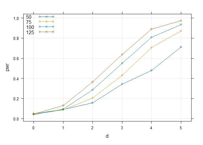
Power curves
Turn into a function of n and effect size
pwrFun <- function(n = 30, d = 4, sd = 10, nrep = 50) {
  n <- n; m <- n
  pval <- replicate(nrep, {
    x <- rnorm(n, mean = 1000 + d, sd = sd)
    y <- rnorm(m, mean = 1000,     sd = sd)
    t.test(x, y, mu = 0, var.equal = TRUE)$p.value
  })
  mean(pval < 0.05)
}
Set up conditions and call power function
cond <- expand.grid(d = 0:5,
                    n = c(50, 75, 100, 125))
cond$pwr <- mapply(pwrFun, n = cond$n, d = cond$d, MoreArgs = list(nrep = 500))

## Plot results
lattice::xyplot(pwr ~ d, cond, groups = n, type = c("g", "b"),
                auto.key = list(corner = c(0, 1)))
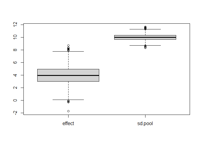
Parameter recovery
n <- 100

out <- replicate(2000, {
  x <- rnorm(n, mean = 1000 + 4, sd = 10)
  y <- rnorm(n, mean = 1000,     sd = 10)
  t <- t.test(x, y, mu = 0, var.equal = TRUE)
  c(
    effect = -as.numeric(diff(t$estimate)),
    sd.pool = t$stderr * sqrt(2*n) / 2
  )
})

rowMeans(out)
##   effect  sd.pool
## 3.978400 9.993142
boxplot(t(out))